Notebook Demo#
We can use Markdown to easily write and style text or make it look like code.
Using LaTeX equations can be done within $$.
Nearfield example#
For a calibration or integration of acoustic data, we should consider ranges at least 3 times (according to Medwin and Clay 1998) the nearfield range (\(r_{nf}\)):
$\(r_{nf} = \frac{\pi d_{t}^2}{4\lambda}\)\(
with wavelength \)\lambda=\frac{c}{f}\( (m) and \)d_t\( (m) is the largest distance across the active elements in a circular piston projector. This recommendataion is about one third more conservative than recommendations found in Simmonds and MacLennan 2005.
With \)\frac{\theta_{-3~dB}}{2}\simeq sin^{-1}(\frac{3.2}{k~d_t})\( with the wave number \)k=\frac{2\pi}{\lambda}$.
Luckily we have already created the uwa package which computes the nearfield of a round transducer at a given frequency, ambient soundspeed and 3 dB beamwidth for us
First let’s check if the uwa package is working as we thing it should:
import uwa #import the uwa package
# create an acoustic wave object
# with an ambient soundspeed of 1470 m/s,
# at 38 kHz with a 3 dB beamwidth of 7°
uw = uwa.AcousticWave(speed =1470, frequency=38e3, bw=7)
#let's see all the results
uw.__dict__
{'frequency': 38000.0,
'speed': 1470,
'bw': 7,
'wl': 0.038684210526315786,
'k': 162.4224773284519,
'ar': 0.32272199776928523,
'rnf': 2.114527228518027}
This is looking good!
Let’s generate a range of values for various frequencies and beamwidths and put them all in a pandas DataFrame:
#import packages
import pandas as pd
#loop over frequencies between 0.1 and 100 kHz and beam widths [3, 20[ °
#NOTE: range in Python includes the starting value but excludes the stop values e.g. range(0,10) is 0,1,2,3,4,5,6,7,8,9
nfs = pd.DataFrame([
uwa.AcousticWave(speed =1470, frequency=f * 100, bw=b).__dict__
for f in range(1,1001)
for b in range(3,20)
])
#let's see the Dataframe
nfs
| frequency | speed | bw | wl | k | ar | rnf | |
|---|---|---|---|---|---|---|---|
| 0 | 100 | 1470 | 3 | 14.7000 | 0.427428 | 286.001578 | 4370.281434 |
| 1 | 100 | 1470 | 4 | 14.7000 | 0.427428 | 214.520243 | 2458.720194 |
| 2 | 100 | 1470 | 5 | 14.7000 | 0.427428 | 171.635802 | 1573.940508 |
| 3 | 100 | 1470 | 6 | 14.7000 | 0.427428 | 143.049809 | 1093.319537 |
| 4 | 100 | 1470 | 7 | 14.7000 | 0.427428 | 122.634359 | 803.520347 |
| ... | ... | ... | ... | ... | ... | ... | ... |
| 16995 | 100000 | 1470 | 15 | 0.0147 | 427.427572 | 0.057357 | 0.175773 |
| 16996 | 100000 | 1470 | 16 | 0.0147 | 427.427572 | 0.053794 | 0.154610 |
| 16997 | 100000 | 1470 | 17 | 0.0147 | 427.427572 | 0.050651 | 0.137070 |
| 16998 | 100000 | 1470 | 18 | 0.0147 | 427.427572 | 0.047858 | 0.122372 |
| 16999 | 100000 | 1470 | 19 | 0.0147 | 427.427572 | 0.045361 | 0.109933 |
17000 rows × 7 columns
Plotting#
We can plot the results interactively, such that we can zoom and get information when hoovering over some points.
import plotly.express as px
import plotly.graph_objects as go
fig = go.Figure()
fig.add_trace(
go.Heatmap()
)
fig.add_trace(
go.Contour(
z=nfs.pivot(index='bw', columns='frequency', values='rnf'),
x=nfs['frequency'].unique() / 1e3,
y=nfs['bw'].unique(),
contours=dict(
coloring ='heatmap',#fill contours like a heatmap
showlabels = True, # show labels on contours
labelfont = dict( # label font properties
size = 12,
color = 'white',
)),
colorbar=dict(
title=dict(
text='Nearfield (m)', # colorbar title
side='right',
font=dict(
size=14,
family='Arial, sans-serif')
)
),
hovertemplate = #stylise the information received when hoovering
"Nearfield: %{z:.2f} m <br>" +
"Frequency: %{x} kHz<br>" +
"3 dB beam width: %{y} °<br>"
)
)
fig.update_traces(colorscale="RdYlBu_r", zmin=1, zmax=10, name="Nearfield (m)")
fig.update_layout(yaxis=dict(title=dict( text="3 dB Beam width (°)" ) ),
xaxis=dict(title=dict( text="Frequency (kHz)" ) ))
fig
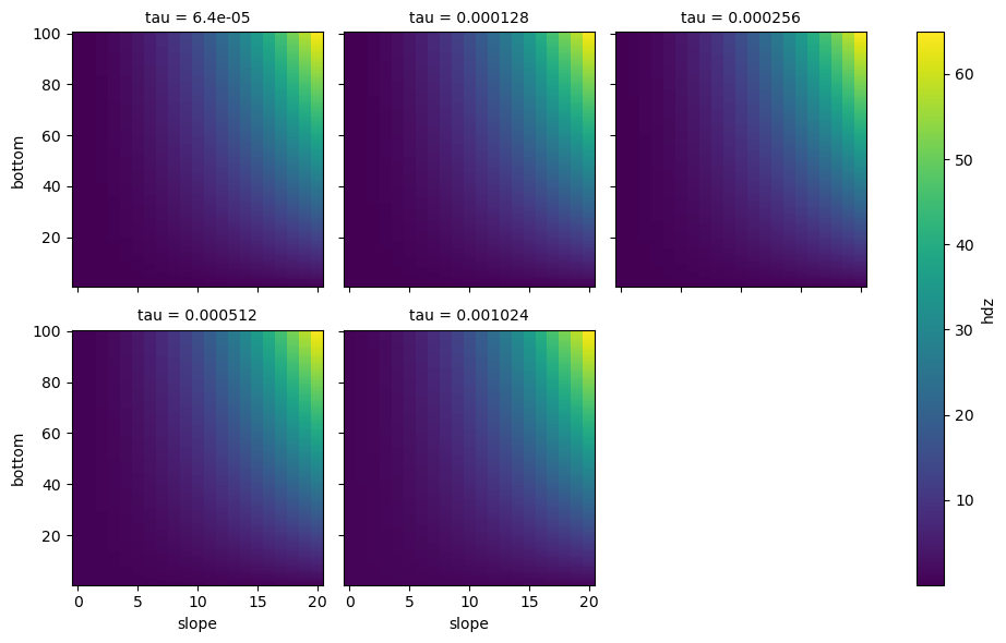
Dead Zone example#
The dead zone depends on the the Bottom depth (m), the bottom slope (°), the pulse duration (s) and the ambient sound speed (m/s). Here we will vary the bottom depth, the slop and the pulse duration to create a multi-dimensional dataset.
import xarray as xr
hdz = xr.Dataset.from_dataframe(
pd.DataFrame([{'bottom':d,'slope':q,'tau':t,'hdz':uwa.deadzone(d=d*10, speed=1460,q=q,tau=t)}
for d in range(1,101) #bottom depth 1 - 100 m
for q in range(0,21) #slope 1 - 41°
for t in [0.001024, 0.000512, 0.000256, 0.000128,0.000064] #pulse duration of 1.024, 0.512, 0.256, 0.128 and 0.64 ms
]).set_index(['bottom','slope', 'tau'])
).to_dataarray(name="hdz")
hdz#.expand_dims("bottom")
<xarray.DataArray 'hdz' (variable: 1, bottom: 100, slope: 21, tau: 5)> Size: 84kB
array([[[[4.67200000e-02, 9.34400000e-02, 1.86880000e-01,
3.73760000e-01, 7.47520000e-01],
[4.82432804e-02, 9.49632804e-02, 1.88403280e-01,
3.75283280e-01, 7.49043280e-01],
[5.28154430e-02, 9.95354430e-02, 1.92975443e-01,
3.79855443e-01, 7.53615443e-01],
...,
[5.61342242e-01, 6.08062242e-01, 7.01502242e-01,
8.88382242e-01, 1.26214224e+00],
[6.22926812e-01, 6.69646812e-01, 7.63086812e-01,
9.49966812e-01, 1.32372681e+00],
[6.88497725e-01, 7.35217725e-01, 8.28657725e-01,
1.01553772e+00, 1.38929772e+00]],
[[4.67200000e-02, 9.34400000e-02, 1.86880000e-01,
3.73760000e-01, 7.47520000e-01],
[4.97665609e-02, 9.64865609e-02, 1.89926561e-01,
3.76806561e-01, 7.50566561e-01],
[5.89108860e-02, 1.05630886e-01, 1.99070886e-01,
3.85950886e-01, 7.59710886e-01],
...
[5.09943220e+01, 5.10410420e+01, 5.11344820e+01,
5.13213620e+01, 5.16951220e+01],
[5.70911944e+01, 5.71379144e+01, 5.72313544e+01,
5.74182344e+01, 5.77919944e+01],
[6.35827148e+01, 6.36294348e+01, 6.37228748e+01,
6.39097548e+01, 6.42835148e+01]],
[[4.67200000e-02, 9.34400000e-02, 1.86880000e-01,
3.73760000e-01, 7.47520000e-01],
[1.99048044e-01, 2.45768044e-01, 3.39208044e-01,
5.26088044e-01, 8.99848044e-01],
[6.56264299e-01, 7.02984299e-01, 7.96424299e-01,
9.83304299e-01, 1.35706430e+00],
...,
[5.15089442e+01, 5.15556642e+01, 5.16491042e+01,
5.18359842e+01, 5.22097442e+01],
[5.76674012e+01, 5.77141212e+01, 5.78075612e+01,
5.79944412e+01, 5.83682012e+01],
[6.42244925e+01, 6.42712125e+01, 6.43646525e+01,
6.45515325e+01, 6.49252925e+01]]]])
Coordinates:
* bottom (bottom) int64 800B 1 2 3 4 5 6 7 8 9 ... 93 94 95 96 97 98 99 100
* slope (slope) int64 168B 0 1 2 3 4 5 6 7 8 ... 13 14 15 16 17 18 19 20
* tau (tau) float64 40B 6.4e-05 0.000128 0.000256 0.000512 0.001024
* variable (variable) object 8B 'hdz'hdz.plot(x="slope", y="bottom", col="tau", col_wrap=3)
<xarray.plot.facetgrid.FacetGrid at 0x298c832a1e0>
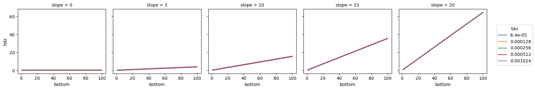
g_simple_line = hdz.isel(slope=slice(0,None,5)).plot(
x="bottom", hue="tau", col="slope", col_wrap=5)
Echogram#
import hvplot.xarray
import panel as pn
mvbs = xr.open_dataset("./python_plotting_files/mvbs.nc")
mvbs
<xarray.Dataset> Size: 6MB
Dimensions: (channel: 4, ping_time: 546, depth: 370)
Coordinates:
* ping_time (ping_time) datetime64[ns] 4kB 2018-03-08T17:37:50 ......
* channel (channel) <U37 592B 'GPT 18 kHz 00907206dc7f 1-1 ES18...
* depth (depth) float64 3kB 0.0 1.0 2.0 3.0 ... 367.0 368.0 369.0
distance (ping_time) float64 4kB ...
Data variables:
Sv (channel, ping_time, depth) float64 6MB ...
latitude (ping_time) float64 4kB ...
longitude (ping_time) float64 4kB ...
frequency_nominal (channel) float64 32B ...
Attributes:
processing_software_name: echopype
processing_software_version: 0.10.0
processing_time: 2025-04-04T14:28:17Z
processing_function: commongrid.compute_MVBS
processing_level: Level 3A
processing_level_url: https://echopype.readthedocs.io/en/stable/p...mvbs.Sv.hvplot(
groupby="channel",
cmap="RdYlBu_r",
x='ping_time',
y='depth',
clim=(-85,-45)).opts(invert_yaxis=True)
mvbs.swap_dims({"ping_time": "distance"}).Sv.hvplot(
groupby="channel",
cmap="RdYlBu_r",
x='distance',
y='depth',
clim=(-85,-45)).opts(invert_yaxis=True)
import holoviews as hv
hv.config.image_rtol = 10000
mvbs.swap_dims({"ping_time": "distance"}).Sv.hvplot(
groupby="channel",
cmap="RdYlBu_r",
x='distance',
y='depth',
clim=(-85,-45)).opts(invert_yaxis=True)