Xarray - Examples#
import xarray as xr
import numpy as np
mvbs = xr.open_dataset("./python_plotting_files/mvbs.nc")
mvbs
<xarray.Dataset> Size: 6MB
Dimensions: (channel: 4, ping_time: 546, depth: 370)
Coordinates:
* ping_time (ping_time) datetime64[ns] 4kB 2018-03-08T17:37:50 ......
* channel (channel) <U37 592B 'GPT 18 kHz 00907206dc7f 1-1 ES18...
* depth (depth) float64 3kB 0.0 1.0 2.0 3.0 ... 367.0 368.0 369.0
distance (ping_time) float64 4kB ...
Data variables:
Sv (channel, ping_time, depth) float64 6MB ...
latitude (ping_time) float64 4kB ...
longitude (ping_time) float64 4kB ...
frequency_nominal (channel) float64 32B ...
Attributes:
processing_software_name: echopype
processing_software_version: 0.10.0
processing_time: 2025-04-04T14:28:17Z
processing_function: commongrid.compute_MVBS
processing_level: Level 3A
processing_level_url: https://echopype.readthedocs.io/en/stable/p...mvbs.Sv.plot(x="ping_time", y="depth", #define axes
col="channel", #define face or columns
col_wrap=2, #how many columns per row
cmap='RdYlBu_r', #colourmap
yincrease=False, # increasing or decreasing y axis
vmin=-85, #colorbar min
vmax=-45 #colorbar max
)
<xarray.plot.facetgrid.FacetGrid at 0x1f4fce06ea0>

Interactive plotting of ´xarray´ datasets is easiest in ´hvplot´
import hvplot.xarray
mvbs.Sv.hvplot(
groupby="channel",
cmap="RdYlBu_r",
x='ping_time',
y='depth',
clim=(-85,-45)).opts(invert_yaxis=True)
Simple Processing#
First we add a linear ´Sv_lin´ to our dataset, to allow for simple operations in linear space:
mvbs = mvbs.assign(Sv_lin = 10**(mvbs.Sv/10))
mvbs
<xarray.Dataset> Size: 13MB
Dimensions: (channel: 4, ping_time: 546, depth: 370)
Coordinates:
* ping_time (ping_time) datetime64[ns] 4kB 2018-03-08T17:37:50 ......
* channel (channel) <U37 592B 'GPT 18 kHz 00907206dc7f 1-1 ES18...
* depth (depth) float64 3kB 0.0 1.0 2.0 3.0 ... 367.0 368.0 369.0
distance (ping_time) float64 4kB ...
Data variables:
Sv (channel, ping_time, depth) float64 6MB -5.398 ... -59.19
latitude (ping_time) float64 4kB ...
longitude (ping_time) float64 4kB ...
frequency_nominal (channel) float64 32B ...
Sv_lin (channel, ping_time, depth) float64 6MB 0.2886 ... 1.2...
Attributes:
processing_software_name: echopype
processing_software_version: 0.10.0
processing_time: 2025-04-04T14:28:17Z
processing_function: commongrid.compute_MVBS
processing_level: Level 3A
processing_level_url: https://echopype.readthedocs.io/en/stable/p...Swap dimensions#
We have ´ping_time´ and ´distance´ that can be used as x axis. In many cases, distance would be preferred, so we swap time for space:
mvbs = mvbs.swap_dims({"ping_time": "distance"})
mvbs
<xarray.Dataset> Size: 13MB
Dimensions: (channel: 4, distance: 546, depth: 370)
Coordinates:
ping_time (distance) datetime64[ns] 4kB 2018-03-08T17:37:50 ... ...
* channel (channel) <U37 592B 'GPT 18 kHz 00907206dc7f 1-1 ES18...
* depth (depth) float64 3kB 0.0 1.0 2.0 3.0 ... 367.0 368.0 369.0
* distance (distance) float64 4kB 0.00475 0.01311 ... 782.3 785.2
Data variables:
Sv (channel, distance, depth) float64 6MB -5.398 ... -59.19
latitude (distance) float64 4kB ...
longitude (distance) float64 4kB ...
frequency_nominal (channel) float64 32B ...
Sv_lin (channel, distance, depth) float64 6MB 0.2886 ... 1.20...
Attributes:
processing_software_name: echopype
processing_software_version: 0.10.0
processing_time: 2025-04-04T14:28:17Z
processing_function: commongrid.compute_MVBS
processing_level: Level 3A
processing_level_url: https://echopype.readthedocs.io/en/stable/p...Rolling mean#
We can apply a rolling mean with a specific window size along time/distance and depth/range:
#Define the window sizes
rm = 2 #range / depth window size
tm = 2 #distance window size
#we use Sv_lin and want to compute a rolling function, here we select mean
ds_mean = mvbs.Sv_lin.rolling(depth=rm, #we wanth the depth dim to be summarised by rm
distance = tm, #we want distance to be summarised y tm
center=True).mean(skipna=True) #we want the mean to be computer
# We do a back transformation into log space
ds_mean = 10 * np.log10(ds_mean)
ds_mean
<xarray.DataArray 'Sv_lin' (channel: 4, distance: 546, depth: 370)> Size: 6MB
array([[[ nan, nan, nan, ..., nan,
nan, nan],
[ nan, -8.4076494 , -50.97955179, ..., -71.91804546,
-68.69957037, -69.56561588],
[ nan, -8.40763162, -50.66636956, ..., -73.27081846,
-73.10200387, -73.17166288],
...,
[ nan, -8.41142378, -50.75877509, ..., -83.60677694,
-83.62927048, -80.98900678],
[ nan, -8.41088802, -50.64022807, ..., -83.54732503,
-84.60018354, -83.63346256],
[ nan, -8.40712569, -51.06284783, ..., -84.87613543,
-85.29087994, -85.30160778]],
[[ nan, nan, nan, ..., nan,
nan, nan],
[ nan, 0.14791044, -41.3800537 , ..., -81.22153272,
-80.79334491, -82.57396961],
[ nan, 0.14595188, -41.39143453, ..., -80.69576775,
-80.08443583, -81.48100564],
...
[ nan, 3.9192607 , -44.40682258, ..., -70.95569039,
-71.70427111, -69.01998705],
[ nan, 3.9195468 , -43.35808353, ..., -71.2566711 ,
-73.74251272, -73.88183955],
[ nan, 3.91991033, -50.01115053, ..., -76.77361869,
-76.90116617, -77.07182198]],
[[ nan, nan, nan, ..., nan,
nan, nan],
[ nan, 8.54430188, -52.69276729, ..., -58.3741028 ,
-57.13750085, -56.12326464],
[ nan, 8.54622877, -53.14282238, ..., -58.70591116,
-58.49576029, -58.21242687],
...,
[ nan, 8.54436095, -49.33292152, ..., -60.02405956,
-58.39513452, -56.31650487],
[ nan, 8.54558151, -47.84906944, ..., -60.08605169,
-60.42404638, -59.9225295 ],
[ nan, 8.54123935, -53.22920332, ..., -58.40156493,
-59.95748037, -60.43446393]]])
Coordinates:
ping_time (distance) datetime64[ns] 4kB 2018-03-08T17:37:50 ... 2018-03-...
* channel (channel) <U37 592B 'GPT 18 kHz 00907206dc7f 1-1 ES18-11' ......
* depth (depth) float64 3kB 0.0 1.0 2.0 3.0 ... 366.0 367.0 368.0 369.0
* distance (distance) float64 4kB 0.00475 0.01311 0.02889 ... 782.3 785.2# and we do a nice interactive plot
ds_mean.hvplot(groupby="channel", #grouping element
cmap="RdYlBu_r", #colormap
x='distance', #x axis
y='depth',#y axis
clim=(-75,-32)).opts(invert_yaxis=True) #colormap limits and inverted y axis
We could ignore the tolerance warning or fix it…
import holoviews as hv
hv.config.image_rtol = 1000
ds_mean.hvplot(groupby="channel",
cmap="RdYlBu_r",
x='distance',
y='depth',
clim=(-75,-32)).opts(invert_yaxis=True)
Median#
We can apply a rolling median with a specific window size along time/distance and depth/range:
rm = 2 #range / depth window size
tm = 10 #distance window size
#we use Sv_lin and want to compute a rolling function, here we select median
ds_median = mvbs.Sv_lin.rolling(depth=rm, #we wanth the depth dim to be summarised by rm
distance = tm, #we want distance to be summarised y tm
center=True).median(skipna=True) #we want the median to be computer
# We do a back transformation into log space
ds_median = 10 * np.log10(ds_median)
# and we do a nice interactive plot
ds_median.hvplot(groupby="channel", #grouping element
cmap="RdYlBu_r", #colormap
x='distance', #x axis
y='depth',#y axis
clim=(-75,-32)).opts(invert_yaxis=True) #colormap limits and inverted y axis
Gaussian Blur#
Another commonly used alorithm is gaussian blur.
We import the ´gaussian_filter´ from the ´scipy.ndimage´ package and apply it:
from scipy.ndimage import gaussian_filter
#Gaussian Blur
sigma=3 #sigma parameter
blur = xr.DataArray(
gaussian_filter(mvbs.Sv_lin, sigma=sigma), #apply gaussian blur to Sv_lin
coords=[mvbs.channel.values, mvbs.distance.values, mvbs.depth.values],
dims=["channel","distance","depth"])
#backtransformation into log space
blur = 10 * np.log10(blur)
# and we do a nice interactive plot
blur.hvplot(groupby="channel", #grouping element
cmap="RdYlBu_r", #colormap
x='distance', #x axis
y='depth',#y axis
clim=(-75,-32)).opts(invert_yaxis=True) #colormap limits and inverted y axis
The world’s most naive and inefficient bottom detection#
from scipy.signal import find_peaks
def get_bottom(sv, data_thresh = -60, bot_thresh = -40, dmax = 200, dmin=50, offset=0.5):
"""
Bottom detection, as primitive as it gets
Attributes:
sv (xarray): MVBS container generated with echopype containing at least Sv values and depth
data_thresh (integer or float): data threshold in dB
bot_thresh (integer or float): minimum value to consider bottom in dB
dmax (integer or float): maximum depth to consider for bottom detection in m
dmin (integer or float): minimum depth to coonsider for bottom detection in m
offset (integer or float): offset from detect bottom line in m
Returns:
xarray.Dataset containing the detected bottom depth in m
"""
bb = []
for ping in sv:
ping = ping.where((ping > data_thresh) & (ping.depth > dmin) & (ping.depth < dmax))
peaks, properties = find_peaks(ping, bot_thresh)
if len(peaks) > 0:
bmax = ping[peaks[np.where(properties['peak_heights']==properties['peak_heights'].max())]]
if bmax > bot_thresh:
bmax = bmax.assign_coords(depth = bmax.depth - offset)
bb.append(bmax)
bot = xr.combine_by_coords(bb)
bot = bot.assign(bottom=bot.depth)
bot = bot.swap_dims({"depth": "distance"})
return(bot)
mvbs = mvbs.assign(blur=blur)
bot = get_bottom(sv=mvbs.blur.isel(channel=1), offset=2, data_thresh=-60, bot_thresh=-30, dmin=100, dmax=400)
bot
<xarray.Dataset> Size: 2kB
Dimensions: (distance: 41)
Coordinates:
ping_time (distance) datetime64[ns] 328B 2018-03-08T17:56:00 ... 2018-03...
channel <U37 148B 'GPT 38 kHz 009072057008 2-1 ES38B'
* distance (distance) float64 328B 785.2 724.9 677.9 ... 47.68 20.61 17.08
depth (distance) float64 328B 124.0 125.0 126.0 ... 162.0 163.0 164.0
Data variables:
blur (distance) float64 328B -17.18 -15.46 -14.87 ... -14.81 -13.81
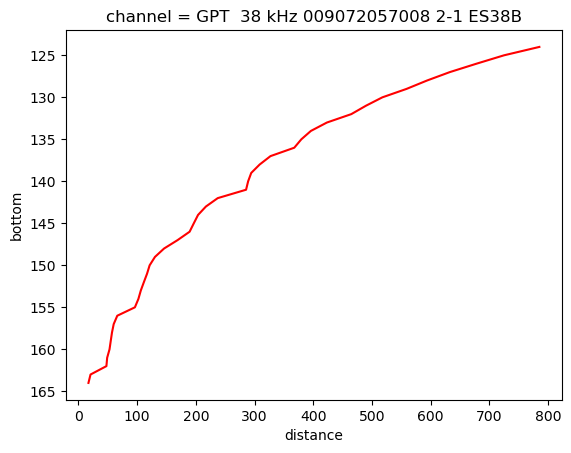
bottom (distance) float64 328B 124.0 125.0 126.0 ... 162.0 163.0 164.0bot.bottom.plot(color='red', yincrease=False)
[<matplotlib.lines.Line2D at 0x21700270650>]
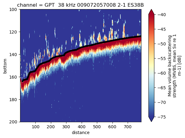
import matplotlib.pyplot as plt
fig, ax = plt.subplots()
mvbs.isel(channel=1).Sv.plot(x='distance', y='depth', vmin=-75, vmax=-40, yincrease=False, ax=ax, cmap='RdYlBu_r')
bot.bottom.plot.line(c='black', ax=ax, linewidth=4)
plt.ylim([200,100])
(200.0, 100.0)